Introduction
This page is all about \(\sum {\bf F} = m \, {\bf a}\), except we will express the forces as stresses acting on differential sized areas. The first example will be 2-D, to minimize the complexity. Then the equations will be developed in 3-D, and also presented in cylindrical coordinates.The concepts and governing differential equations of equilibrium derived here are vital to finite element theory. Pay close attention!
2-D Equilibrium
The 2-D differential object is shown in the sketch at the right. The idea is to sum all the forces on it and set them equal to \(m \, {\bf a}\). This can be done one component at a time, so start with the x-direction. The forces consist of
- \(\sigma_{xx}\) acting on face \(dy\) in the \(-x\) direction
- \(\tau_{xy}\) acting on face \(dx\) in the \(-x\) direction
- \(\sigma_{xx} + {\partial \sigma_{xx} \over \partial x} dx\) acting on face \(dy\) in the \(+x\) direction
- \(\tau_{xy} + {\partial \tau_{xy} \over \partial y} dy\) acting on face \(dx\) in the \(+x\) direction
- Plus "body forces". These include any forces due to gravity, magnetism, etc, and are summarized simply as \(\rho f_x dx dy\) where \(f_x\) is force per unit mass
Acceleration is simply \(a_x\), although it is perfectly permissible to use the material derivative: \({\partial v_x \over \partial t} + v_x {\partial v_x \over \partial x}\).
Summing all this up gives
\[ -\sigma_{xx}dy - \tau_{xy}dx + \left( \sigma_{xx} + {\partial \sigma_{xx} \over \partial x} dx \right) dy + \left( \tau_{xy} + {\partial \tau_{xy} \over \partial y} dy \right) dx + \rho f_x dx dy = \rho \, dx dy \, a_x \]
Cleaning up terms that cancel, and dividing through by \(dx dy\) gives
\[ {\partial \sigma_{xx} \over \partial x} + {\partial \tau_{xy} \over \partial y} + \rho f_x = \rho \, a_x \]
And summing forces in the y-direction leads to
\[ {\partial \sigma_{yy} \over \partial y} + {\partial \tau_{xy} \over \partial x} + \rho f_y = \rho \, a_y \]
It is interesting how the equations tie together changes in all the different stress components, making them interdependent on each other.
An object is said to be in equilibrium when the right hand sides (RHS) of the equations are zero.
3-D Equilibrium
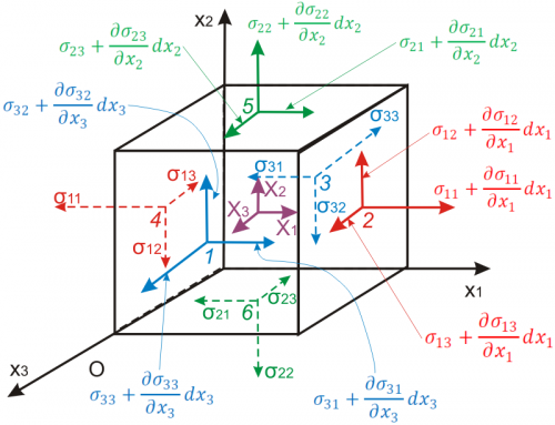
The forces consist of
- \(\sigma_{11}\) acting on face \(dx_2 dx_3\) in the \(-x\) direction
- \(\sigma_{21}\) acting on face \(dx_1 dx_3\) in the \(-x\) direction
- \(\sigma_{31}\) acting on face \(dx_1 dx_2\) in the \(-x\) direction
- \(\sigma_{11} + {\partial \sigma_{11} \over \partial x_1} dx_1\) acting on face \(dx_2 dx_3\) in the \(+x\) direction
- \(\sigma_{21} + {\partial \sigma_{21} \over \partial x_2} dx_2\) acting on face \(dx_1 dx_3\) in the \(+x\) direction
- \(\sigma_{31} + {\partial \sigma_{31} \over \partial x_3} dx_3\) acting on face \(dx_1 dx_2\) in the \(+x\) direction
- The body force is \(\rho f_x dx_1 dx_2 dx_3\) where \(f_x\) is force per unit mass
The mass is density times volume: \(\rho \, dx_1 dx_2 dx_3\).
Acceleration is simply \(a_x\), although it is perfectly permissible to use the material derivative: \({\partial v_x \over \partial t} + v_x {\partial v_x \over \partial x}\).
Summing all this up gives
\[ {\partial \sigma_{11} \over \partial x_1} dx_1 dx_2 dx_3 + {\partial \sigma_{21} \over \partial x_2} dx_1 dx_2 dx_3 + {\partial \sigma_{31} \over \partial x_3} dx_1 dx_2 dx_3 + \rho f_x = \rho \, dx_1 dx_2 dx_3 a_x \]
Dividing through by the differential volumes gives
\[ {\partial \sigma_{11} \over \partial x_1} + {\partial \sigma_{21} \over \partial x_2} + {\partial \sigma_{31} \over \partial x_3} + \rho f_x = \rho \, a_x \]
And since the stress tensor is symmetric...
\[ {\partial \sigma_{11} \over \partial x_1} + {\partial \sigma_{12} \over \partial x_2} + {\partial \sigma_{13} \over \partial x_3} + \rho f_x = \rho \, a_x \]
The complete set of equations is
\[ {\partial \sigma_{11} \over \partial x_1} + {\partial \sigma_{12} \over \partial x_2} + {\partial \sigma_{13} \over \partial x_3} + \rho f_x = \rho \, a_x \] \[ {\partial \sigma_{21} \over \partial x_1} + {\partial \sigma_{22} \over \partial x_2} + {\partial \sigma_{23} \over \partial x_3} + \rho f_y = \rho \, a_y \] \[ {\partial \sigma_{31} \over \partial x_1} + {\partial \sigma_{32} \over \partial x_2} + {\partial \sigma_{33} \over \partial x_3} + \rho f_z = \rho \, a_z \]
All this is written in matrix and tensor notation as
\[ \nabla \cdot \boldsymbol{\sigma} + \rho \, {\bf f} = \rho \, {\bf a} \qquad \qquad \sigma_{ij,j} + \rho f_i = \rho \, a_i \]
Or one could write the acceleration as the material derivative.
\[ \nabla \cdot \boldsymbol{\sigma} + \rho \, {\bf f} = \rho \, \left( {\partial {\bf v} \over \partial t} + {\bf v} \cdot {\partial {\bf v} \over \partial {\bf x}} \right) \qquad \qquad \sigma_{ij,j} + \rho f_i = \rho \, ( v_{i,t} + v_k v_{i,k} ) \]
Equilibrium in Cylindrical Coordinates
The equilibrium equations in cylindrical coordinates contain several additional terms, such as \({\sigma_{\theta \theta} \over r}\) and \({\sigma_{\theta z} \over r}\), that further complicate matters.\[ \begin{eqnarray} & & {1 \over r} {\partial \over \partial \, r} \left( r \sigma_{rr} \right) + {1 \over r} {\partial \, \sigma_{\!r\theta} \over \partial \, \theta} + {\partial \, \sigma_{\!rz} \over \partial z} - { \sigma_{\!\theta\theta} \over r} + \rho f_r = \rho \, a_r \\ \\ \\ & & {1 \over r} {\partial \over \partial \, r} \left( r \sigma_{r \theta} \right) + {1 \over r} {\partial \, \sigma_{\!\theta\theta} \over \partial \, \theta} + {\partial \, \sigma_{\!\theta z} \over \partial z} + {\sigma_{\!r \theta} \over r} + \rho f_\theta = \rho \, a_\theta \\ \\ \\ & & {1 \over r} {\partial \over \partial \, r} \left( r \sigma_{rz} \right) + {1 \over r} {\partial \, \sigma_{\!\theta z} \over \partial \, \theta} + {\partial \, \sigma_{\!zz} \over \partial z} + \rho f_z = \rho \, a_z \end{eqnarray} \]
Centripetal Acceleration
It is possible to get a quick, rough estimate of the circumferential stress level in a tire undergoing axisymmetric centripetal forces during a high speed limit test. The radial acceleration equation is\[ {1 \over r} {\partial \over \partial \, r} \left( r \sigma_{rr} \right) + {1 \over r} {\partial \, \sigma_{\!r\theta} \over \partial \, \theta} + {\partial \, \sigma_{\!rz} \over \partial z} - { \sigma_{\!\theta\theta} \over r} + \rho f_r = \rho \, a_r \\ \]
The radial acceleration is
\[ a_r = - {V^2 \over r} \]
The other terms are expected to be negligible, except \(\sigma_{\theta\theta} / r\). Setting these two equal to each other gives
\[ - {\sigma_{\theta\theta} \over r} = - \rho {V^2 \over r} \]
This simplifies to
\[ \sigma_{\theta\theta} = \rho V^2 \]
So for a tire spinning at 200 kph (= 55.55 m/s), with rubber density equal to 1,150 kg/m3, the circumferential stress should be around
\[ \sigma_{\theta\theta} \; = \; (1150 \text{ kg/m}^3) (55.55 \text{ m/s})^2 \; = \; 3,500,000 \text{ Pa} \; = \; 3.5 \text{ MPa} \]
For the steel in the NSTs, the density is 7,800 kg/m3, and the circumferential stress should be around
\[ \sigma_{\theta\theta} \; = \; (7800 \text{ kg/m}^3) (55.55 \text{ m/s})^2 \; = \; 24,000,000 \text{ Pa} \; = \; 24 \text{ MPa} \]
The fact that the tire is actually a nonhomogeneous composite probably makes the actual values significantly different from these estimates.
Steel Belt Equilibrium
This example relates interply shear strain, \(\gamma_{xz}\), which is present between the steel belts and peaks at the belt edge, to intraply shear stress, \(\tau_{xy}\), in the plane of the belts.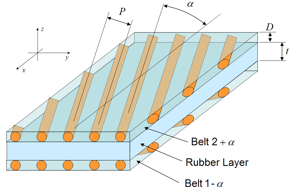
The main governing equilibrium equation for this situation is
\[ {\partial \sigma_{xx} \over \partial x} + {\partial \tau_{xy} \over \partial y} + {\partial \tau_{xz} \over \partial z} + \rho f_x = \rho \, a_x \]
Assume that several terms in the equation are negligible, leaving only
\[ {\partial \tau_{xy} \over \partial y} + {\partial \tau_{xz} \over \partial z} = 0 \]
The interply rubber layer develops shear, called \(\gamma_{xz}\). Therefore the shear stress is
\[ \tau_{xz} = G \gamma_{xz} \]
Now focus on the top belt. The shear stress, \(\tau_{xz}\), in the shear layer is the shear stress on the bottom surface of the belt. But the shear stress on the top is near zero. So the change in shear stress through the thickness of the belt is
\[ {\partial \tau_{xz} \over \partial z} \; = \; {\tau_\text{top} - \tau_\text{bottom} \over D} \; = \; {0 - G \gamma_{xz} \over D} \; = \; -\left( { G \over D}\right) \gamma_{xz} \]
Substituting this into the equilibrium equation gives
\[ {\partial \tau_{xy} \over \partial y} - \left( { G \over D}\right) \gamma_{xz} = 0 \]
So the intraply shear in the belt can be related to the interply shear strain as
\[ \tau_{xy} = \int \left( { G \over D}\right) \gamma_{xz} \, dy \]
Granted, this equation my not be very useful by itself. But it is essential to the general analytical solution for the stresses and strains in the belts.